Lifetime value (LTV) targeted per customer

Estimating each customer’s LTV, rather than an average per category, lets CRM effort be concentrated on the most profitable customers, and lets you pay more to acquire those whose LTV is high.

Introduction

Lifetime value (LTV) is a key KPI in digital marketing. LTV is a customer’s value, and therefore the most a company can afford to pay to acquire a new customer while staying profitable. It therefore lets digital marketing tools be steered so as to acquire only profitable customers, and so to maximise profit.

Traditionally, marketing strategies rest on average LTVs. Since a specific customer’s value is hard to quantify at the moment of their first purchase, an average value per category, or by acquisition source, is calculated beforehand and given to each customer by their category. Some customers will prove better than their category’s average, while others will be less profitable. On the whole, however, newly acquired customers should have a value close to the average calculated. In that case our approximation is effective from a profitability point of view.

More complex and a little less intuitive as it is, the individual LTV model we use, presented in the paragraphs below, has several advantages over simpler methods — notably from a customer engagement point of view.

Being able to estimate the LTV of each customer, for instance, lets us concentrate CRM effort on the most profitable ones.

The method, and some of its possible applications, are explained and set out in this article.

How it works

To calculate an individual LTV for each customer, we need all the transactions they made. The model we built works with three elements:

• Frequency: the time between two transactions
• Recency: the time since the last transaction
• The amount of the transaction

Frequency and recency let a probability of attrition be calculated. Against the recency and the average frequency of the customer studied, a probability is assigned. It reflects the chances that the customer is still active with the company. A complete explanation of that concept is available in one of our earlier articles.

In parallel, an estimated average basket is calculated per customer. It estimates the average basket value across every transaction, past and future, that a particular customer will make. The estimated average basket is calculated from three elements:

• The number of purchases that customer made
• That customer’s observed average basket (total spend / number of purchases)
• The distribution of the average basket across all customers

First, the distribution of the average basket across all customers is estimated.

A single purchase at 100 CHF leaves Toto’s estimated basket at 53 CHF; it takes ten to bring it to 92 CHF

Density of the average basket across all customers, in CHF, and Toto’s estimated average basket — Toto spends 100 CHF on every purchase. Move the number of purchases.

Toto’s purchases at 100 CHF: 1

1 purchase 2 purchases 5 purchases 10 purchases

Grey dots: the estimate after 1, 2, 5 and 10 purchases, the article’s reference points. Curve: a gamma distribution of shape 9 and scale 6 (mode 48 CHF, mean 54 CHF), fitted to the article’s figure. Estimated basket: a weighted average between 53.34 CHF, the estimate after a single purchase, and the observed basket of 100 CHF; the weight of the observed basket is (n − 1) / (n − 1 + 1.89) for n purchases, the shape of the gamma-gamma model. It passes through the article’s four points.

Source: the article’s example (fictional customer “Toto”); curve and points read off its original figure, approximate values · Chart: bright.swiss

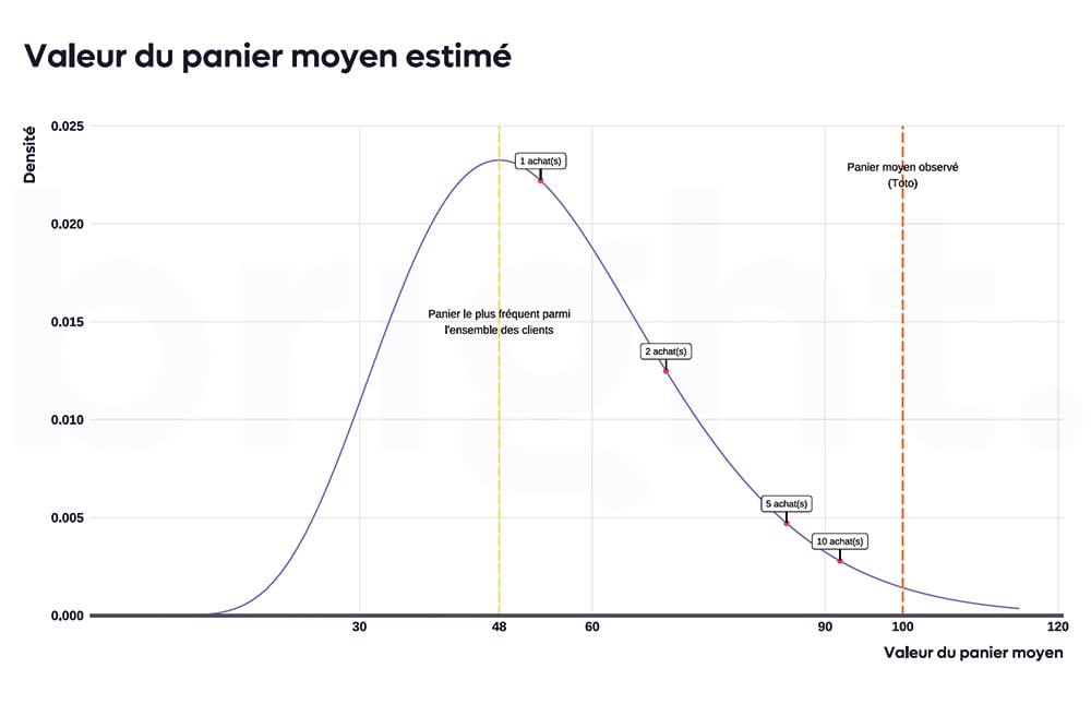
In chart 1 it is in purple. We can see that the average basket of a randomly chosen customer most often sits around CHF 48.

Imagine the basket of customer Toto’s first purchase is CHF 100 (the vertical red line). It is not because their first basket is CHF 100 that every purchase they then make will be CHF 100. The overall distribution says rather that the average basket of a randomly chosen customer is CHF 48. Because their first purchase is significantly above the average basket, however, the model will estimate Toto’s average basket at CHF 53.34, reflecting the probability that they will spend more than a randomly chosen customer.

The method pulls their estimated average basket towards the most likely value, by their purchasing behaviour. The more transactions Toto makes at CHF 100, the more we deduce that their estimated average basket is close to CHF 100. After ten transactions at CHF 100, for instance, we estimate Toto’s average basket at CHF 91.91.

The method used to estimate a customer j’s average basket is relatively intuitive. When customer j makes few transactions, the method pulls their estimated average basket towards the most frequently observed average basket, estimated across all customers. The more transactions customer j makes, the more their basket reflects their real purchasing behaviour and moves away — or not — from the average estimated across all other customers.

The higher the number of transactions, the more certain we are about customer j’s behaviour on the transactions to come. That phenomenon is shown by the pink dots — the estimated average basket — moving along the purple curve against the observed average as the number of transactions rises, in chart 1 (Toto’s example).

Finally, we combine the theoretical average basket with the probability of attrition, to obtain an LTV per customer. Two interesting points of view can then be taken, depending on the need:

1. The remaining LTV of a customer over a given period can be estimated.
   • Example: by their past activity, we estimate that customer Toto will spend a further CHF 100 over the next three years.
2. From there, a customer’s total LTV over a defined period can be calculated.
   • Toto has been a customer for two years and has spent CHF 200 since arriving. We estimated they will spend a further CHF 100 over the next three years. Their total value is therefore CHF 300 at five years.

The first point of view is rather useful for improving your CRM mechanics, while the second serves more for acquisition.

LTV and customer engagement

It is key to understand clearly that a good past customer is not the same as a good future customer. A customer may have been very profitable in the past, but if they have not transacted for a long time we will conclude that they have churned — they will have a very high probability of attrition. In that case the customer is of little interest from a CRM point of view, because the remaining LTV will be small.

On the other side, a customer who has made only two high-margin purchases since registering, and whose recency is short, will likely be considered promising. That kind of customer deserves particular attention from the CRM team, because it is customers like that who should generate the company’s future profit.

The CRM team will therefore concentrate its effort on the customers with the highest remaining LTVs. Among the possible actions, it could:

• Vary the newsletters by the customer’s quality.
• Prioritise tickets or after-sales requests by the customer’s quality.
• Interact more with the customers of high remaining LTV

The idea is to give them particular attention so that they do not churn, since they will contribute strongly to profit in the short and medium term.

Remarketing

Remarketing is an area where remaining LTV can be very useful. It is sensible to target customers with high remaining LTVs, because we know they are the ones most likely to buy again.

LTV and acquisition

LTV per customer also lets us assess the optimal price we can afford to invest in acquiring a new customer.

In that case we have to consider total LTV. A customer’s cost has to be set against the LTV they will bring across their whole journey. The total LTVs of customers already acquired let us calculate that value.

The total LTVs of recent customers will be estimated over a given period — five years, for instance. The average of those LTVs is the maximum price payable for a new customer.

Segmentation

To make our customer acquisition strategy more effective, a segmentation based on behaviour can be applied, so as to fit the bids to the target better.

The idea underlying that practice is that every customer, as long as their margin is positive, should be acquired. The optimisation comes from varying the acquisition costs. We can afford to pay more to acquire a customer if we judge their LTV to be high. When the bids are fitted to the customer’s quality, profit rises.

For segmentation we can use the marketing channels’ own algorithms, or do it ourselves. An explanation of each case follows:

Facebook lookalike

Using Facebook’s lookalike feature can make for effective segmentation, drawing on Facebook’s craft. The concept is this:

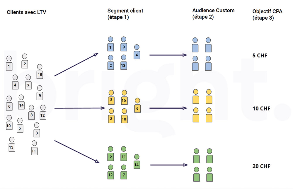
1. We create segments grouping people with more or less similar total LTVs (step 1 in chart 2).
2. Each segment is passed to Facebook as a “Custom Audience”. Facebook uses it to acquire similar customers (step 3 in chart 2).
3. Each “Custom Audience” has a different bid (step 3 in chart 2).

That way Facebook agrees to acquire high-value customers at higher prices, while being tighter for less profitable ones. Chart 2 below illustrates the point.

One LTV segment, one audience, one bid: high-value customers are acquired at a higher price

LTV segmentation passed to Facebook, in three steps, for fifteen example customers (figure 2 of the article). Choose a segment or a step.

5 CHF target 10 CHF target 20 CHF target

Source: the article’s diagram (figure 2), customers numbered as in the original · Chart: bright.swiss

What is remarkable about this method is that Facebook takes care of identifying which factors influence a customer’s quality, with nothing for us to do. What is more, Facebook may know more about the customer than we as a company do. Through its data, its algorithms could prove more effective than an analysis carried out on our side.

That strategy is presented with Facebook as the marketing channel, but it generalises to others, such as Google.

Regression

Alternatively, we could decide to identify the characteristics that influence LTV ourselves. One possible method would be a regression, so as to identify the factors strongly correlated with LTV.

That has the advantage that we know which factors influence LTV, and by how much. That knowledge can then be used across the various marketing channels to improve the acquisition strategies. It contrasts with the “black box” algorithms of Facebook or Google.

The strengths of that method are better visibility of the factors that matter to LTV, and being able to include the whole of the customer master data available in the regression — information not necessarily available to the marketing channels.

Business insight

Beyond the uses described above, LTV per customer also has the advantage of giving information about the business’s current health, and of offering some interesting perspectives. We propose two charts below.

Dependence on good customers

In general, it is fundamental to know which part of the customer base generates most of the margin. Depending on the business model, fewer than 10% of customers may sometimes make the great majority of the company’s profit. The more a company depends on a few customers for its profit, the more at risk it is should it lose a customer of high LTV. Individual LTV can help represent that situation, because it allows a fair comparison between customers.

At the average CPA of 200 CHF, only 3 customers in 10 are profitable

Five-year LTV of each quantile of customers, ordered from least to most profitable, in CHF, against the acquisition cost (CPA) paid per customer. Move the CPA.

CPA paid per customer: 200 CHF

The article’s average CPA: 200 CHF

Each point on the curve is the LTV of the customer at that quantile. The original curve stops at the 99^th percentile.

Source: the article’s data, read off its original figure, approximate values (±5 CHF) · Chart: bright.swiss

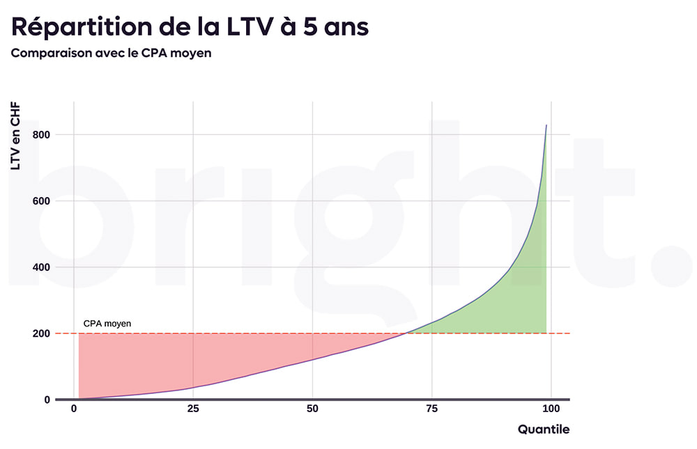
Reading chart 3, we see that 70% of customers are not profitable (we assume every customer was acquired through paid marketing). The grey area, the loss tied to unprofitable customers — those whose lifetime value is below the average CPA — should cover a smaller surface than the blue one, the profitable customers.

On this chart we see, for instance, that only the best 30% of customers acquired have a value above the average CPA paid. Those 30% therefore have to be profitable enough to cover the loss on the 70% who are not, and to pay the company’s fixed costs — salaries, rent and so on.

What is more, we can see that the best customers are not good enough to generate a very large share of the margin on their own. The best 10% are responsible for 32% of the margin.