Calculating a sound conversion rate

Calculating a sound conversion rate

Thomas Boyer
November 22, 2022 · 9 min

Dividing conversions by leads underestimates the conversion rate, because some leads have not yet had time to convert. Bringing each lead’s observation time into the calculation corrects it — and with it the CPL.

Swipe left to read

Keep reading

Back to all our articles

Context

The conversion rate is an essential value for measuring how effective your conversion funnel is. It shows which stage of the funnel causes trouble in the move from lead to customer, and lets a more fitting CPL be set.

Unfortunately, that measure is often calculated wrongly, using the formula #conversions/#leads. The bias of that method is that it does not take into account that some of the leads observed have not had enough time to convert. In certain cases the difference can be very large.

Example:

Suppose we have 50 leads with a maturity of one year — they became leads a year ago — and that over time all of them became customers, with a time to conversion of between two and eight months.
Suppose also that we have 50 leads, less mature, with a maturity of less than a month. Those leads have not converted so far.

A single glance at that situation is enough to deduce that the 50 immature leads simply have not had time to convert, and will probably convert between the second and eighth month like their predecessors. The conversion rate would therefore be 100%.

Yet the traditional conversion rate calculation above ignores that and applies:
Conversion rate = 50/(50+50) = 50%

That extreme example is representative of the underestimation that appears when the conversion rate is calculated that simply.

To avoid it, each lead’s observation time has to be built into the calculation. It is the same precaution as in calculating the average LTV across many cohorts: count only what has had time to be observed.

The bright method

Vocabulary

So that the rest of the article reads more easily, a short glossary:

Lead = a prospect who is not yet a customer (someone who created an account but has not generated margin for the company so far)
Customer = a lead who has made a purchase.
Convert = to move from lead to customer. To make a purchase.
Distance = the time between a lead’s or customer’s registration and the date of observation. That is the lead’s or customer’s observation time.
Period = for a customer, the time between registration and conversion. For a lead that measure does not exist.
CPL = cost per lead
CPA = cost per acquisition (cost per customer)
Cohort = the month a lead was acquired

Introduction

The conversion rate at time t is the probability that a lead converted before, or exactly at, time t. We write it:

$Q_{t} = P (Period \leq t)$

The conversion rate is then the limit, as t tends to infinity, of $lim_{t \to \infty} Q_{t}$ .

In practice the conversion rate settles far sooner, of course, and we can be satisfied with calculating Qt for a t large enough that the conversion rate stops rising.
Once those values are calculated, we know not only the final conversion rate but also the time needed to convert.

Here is an example of the usual shape of the conversion rate over time:

Conversion rate curve: a quick rise, which then flattens.

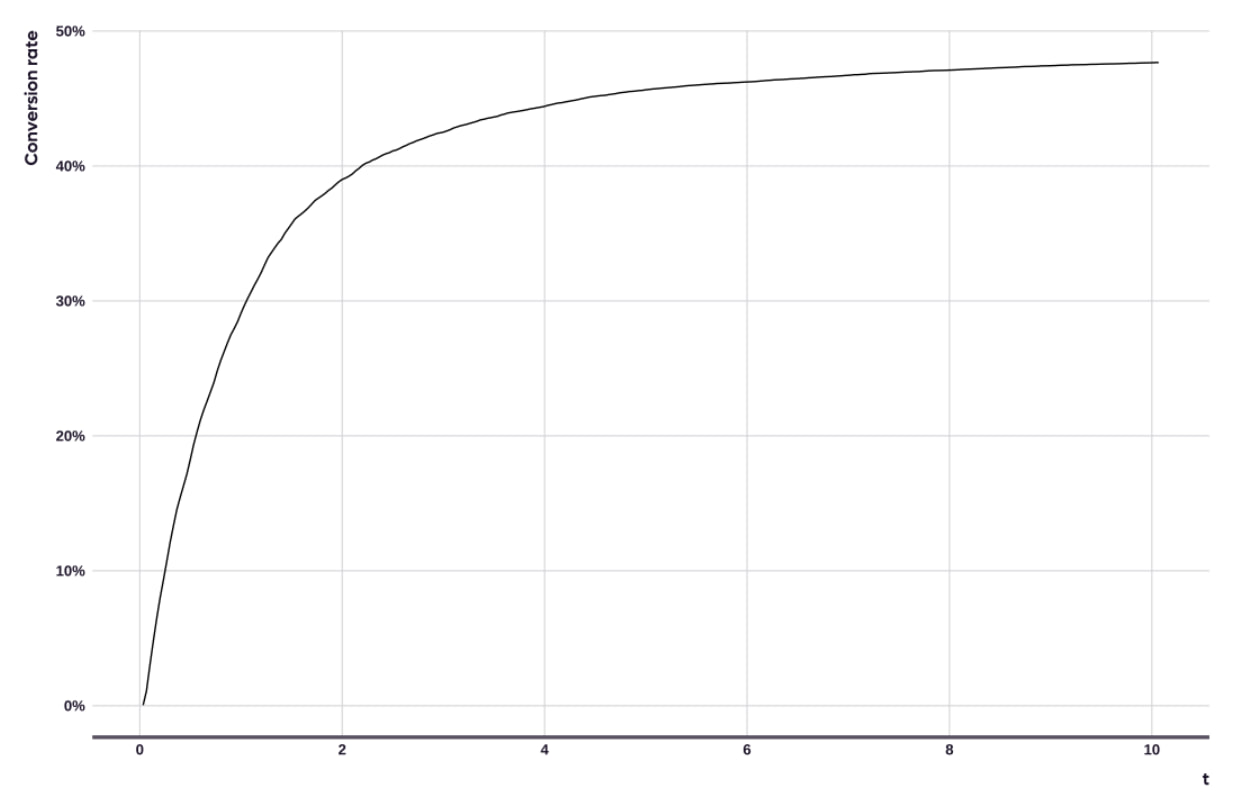
The curve’s shape is generally concave — it flattens over time. That means the more time passes, the less likely a lead is to convert at exactly the present moment. In this example the curve seems to flatten slightly below 50%. That is our final conversion rate.

Most of the time the data is mature enough to see the moment the curve flattens. For young companies, however, there are projection methods — which we will not cover here — for extending the curve.

A probabilistic approach

The aim of this chapter is to set out how the Qt are calculated — the probability of having converted at time t.

Method

First, to simplify the calculation, time has to be made discrete. Instead of treating time as a continuous variable, we break it into whole numbers representing the number of time units elapsed. In practice we use days, but the calculation holds for any unit — week, month, quarter and so on. It is then enough to calculate Qt for every natural number t.

To that end we calculate, for every n ∊ {0,1,2,3,…}, the probability that a lead that has not yet converted converts at exactly time n. Call that probability $p_{n}$ .

We can then calculate Qt from the pn, cumulatively, through the formula:

$Q_{t} = 1 - \overline{Q_{t}} = 1 - \prod_{n = 0}^{t} \overline{p_{n}} = 1 - \prod_{n = 0}^{t} (1 - p_{n})$

Calculating the pn

They are estimated by calculating the proportion of conversions at exactly time n among the observed leads that have not yet converted.

Numerator: the number of leads converting at exactly time n.
Denominator: the number of leads meeting the following conditions:
Distance ≽ n: the lead is mature enough to be observed at time n
Not having Period < n: the lead has not converted
$p_{n}$ = numerator / denominator

A simple example

Here is a small-scale example of the method above:

We observe five leads with their respective distances and periods. For the leads that have not converted (so far), the period is noted NA:

Five customer silhouettes, each with its period and its purchase distance.

Through the formulas above we can calculate the parameters pn and Qn.

At time 1 we observe five people; only one converted at exactly time 1.
p1 = 1/5 = 0.2 and Q1 = 1−(1−p1) = 1−0.8 = 0.2
At time 2 we observe four people. One of them has already converted, so only three are in a position to convert. None converted at exactly time 2.
p2 = 0/3 = 0 and Q2 = 1−(1−p1)(1−p2) = 1−0.8×1 = 0.2
At time 3 we observe three people. One of them has already converted, so only two are in a position to convert. One of them converted at exactly time 3.
p3 = 1/2 = 0.5 and Q3 = 1−(1−p1)(1−p2)(1−p3) = 1−0.8×1×0.5 = 0.6

Still with us? Good — we can gather those figures in a summary table:

t (time)	Numerator	Denominator	Pt	Qt
1	1	5	0.2	0.2
2	0	3	0	0.2
3	1	2	0.5	0.6

The final conversion rate by this method is therefore 60% (3/5), against 40% (2/5) had we used the standard method.

That is because, by our model, p3 = 0.5: of two individuals able to convert at that time, there is one conversion. So there is a one-in-two chance of converting at exactly time 3.

The interpretation is that among individuals 2 and 5, who are not mature, we forecast that one of the two will convert at time 3.

Towards an optimal use of the conversion rate

A good theoretical grasp of probability lets us build a conversion rate calculation that is simple and elegant. Here are some of the insights it gives us.

Setting a fitting CPL

Suppose we already know the acquisition cost (CPA) we want for a new customer. Unfortunately, in running campaigns, our KPIs — the CPL in particular — will be defined against the leads generated, and not against customers; that is so the campaign can be optimised quickly, which would not be possible if we had to wait several months for the leads to become customers.

The conversion rate, calculated properly, nonetheless ties the CPA and the CPL together through the formula CPL = CPA × conversion rate.

As shown above, the naive #customers/#leads calculation would make us underestimate the conversion rate and then the optimal CPL. By setting the CPL too low we would be under-investing against the optimum, and we would miss opportunities.

A better conversion rate calculation therefore corrects the CPL, and so brings better campaign results.

Going further (yes, we can): leads can be segmented — by acquisition channel, by socio-demographic data and so on — and the calculation applied to each of those segments, so as to assess whether one group is more likely to convert than another.
It is common, for instance, for the conversion rate to differ between acquisition channels. You then have to:

Put a tracking system in place
Segment the leads by acquisition channel
Calculate the conversion rate for each segment
Fit the CPL per channel

Improving your conversion funnel

Where the conversion funnel has several stages, the calculation can be adapted to see the conversion rate between each stage of the funnel.
That information then lets a potential bug in the funnel be detected, or the next improvement efforts be better directed.

Case study: assessing marketing performance more effectively

This example is far more complex than the others, but is meant to illustrate the conversion rate’s potential. Some calculations are not fully explained, so that the article stays concise.

Suppose we are a company, and that from May 2022 we tested a different campaign mix, twice as expensive but generating far more leads, at a similar CPL. At first sight that looks an excellent way of raising volume sharply without over-investing, since the CPL seems unaffected.

To challenge that, we can look at the projected conversion rate by cohort — the month the lead was acquired. Here we skip some very interesting steps of the calculation that fall outside this article’s scope, notably how to project a cohort’s future conversions from the conversion rate, and so obtain the projected conversion rate per cohort.

Bar chart of leads by month, overlaid with a curve: volume and quality do not move together.

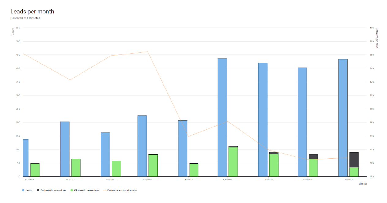
In this chart we see that there was indeed a strong rise in the number of leads since the new marketing mix launched in May (the height of the bars).

In black we have the number of conversions observed, and in blue the conversions to come, estimated through our conversion rate calculation. Note that the closer the month is to the present, the less mature the leads observed. That is why, on the right of the chart, the blue — estimated conversions — dominates.

From this we get the conversion rate per cohort, through the calculation
#projected conversions/#leads (possible because the number of conversions is projected).

We then compare the four months with the old marketing mix against the four months with the new one.

There is indeed a large rise in the number of leads: from 799 to 1,693, a rise of 112%. That would justify doubling the marketing spend, since the number of leads more than doubled.
It is less clear, however, looking at the projected number of customers (projecting matters, or the figures are not comparable): from 255.9 to 378.8, a rise of 48%. In reality the new campaigns generate more leads, but of poorer quality than the old ones. The conversion rate is therefore far lower.

So what at first looked like excellent performance proves, through the conversion rate, to be a mistake that must be corrected quickly: we are spending twice the budget to raise the number of customers by only 48%. One way of putting it is that the new customers generated are worth twice the old ones.

The moral is that the CPL is not necessarily proportional to the CPA. In the face of large changes, the impact has to be watched across several metrics — the conversion rate in particular — so as to have the complete picture.